Bivariate analysis of continuous and/or categorical variables

Tidycomm includes five functions for bivariate explorative data analysis:

crosstab() for both categorical independent and dependent variables
t_test() for dichotomous categorical independent and continuous dependent variables
unianova() for polytomous categorical independent and continuous dependent variables
correlate() for both continuous independent and dependent variables
regress() for both continuous or factorial (translated into dummy dichotomous versions) independent and continuous dependent variables

We will again use sample data from the Worlds of Journalism 2012-16 study for demonstration purposes:

WoJ
#> # A tibble: 1,200 × 15
#>    country   reach employment temp_contract autonomy_selection autonomy_emphasis
#>    <fct>     <fct> <chr>      <fct>                      <dbl>             <dbl>
#>  1 Germany   Nati… Full-time  Permanent                      5                 4
#>  2 Germany   Nati… Full-time  Permanent                      3                 4
#>  3 Switzerl… Regi… Full-time  Permanent                      4                 4
#>  4 Switzerl… Local Part-time  Permanent                      4                 5
#>  5 Austria   Nati… Part-time  Permanent                      4                 4
#>  6 Switzerl… Local Freelancer NA                             4                 4
#>  7 Germany   Local Full-time  Permanent                      4                 4
#>  8 Denmark   Nati… Full-time  Permanent                      3                 3
#>  9 Switzerl… Local Full-time  Permanent                      5                 5
#> 10 Denmark   Nati… Full-time  Permanent                      2                 4
#> # ℹ 1,190 more rows
#> # ℹ 9 more variables: ethics_1 <dbl>, ethics_2 <dbl>, ethics_3 <dbl>,
#> #   ethics_4 <dbl>, work_experience <dbl>, trust_parliament <dbl>,
#> #   trust_government <dbl>, trust_parties <dbl>, trust_politicians <dbl>

Compute contingency tables and Chi-square tests

crosstab() outputs a contingency table for one independent (column) variable and one or more dependent (row) variables:

WoJ %>% 
  crosstab(reach, employment)
#> # A tibble: 3 × 5
#>   employment Local Regional National Transnational
#> * <chr>      <dbl>    <dbl>    <dbl>         <dbl>
#> 1 Freelancer    23       36      104             9
#> 2 Full-time    111      287      438            66
#> 3 Part-time     15       32       75             4

Additional options include add_total (adds a row-wise Total column if set to TRUE) and percentages (outputs column-wise percentages instead of absolute values if set to TRUE):

WoJ %>% 
  crosstab(reach, employment, add_total = TRUE, percentages = TRUE)
#> # A tibble: 3 × 6
#>   employment Local Regional National Transnational Total
#> * <chr>      <dbl>    <dbl>    <dbl>         <dbl> <dbl>
#> 1 Freelancer 0.154   0.101     0.169        0.114  0.143
#> 2 Full-time  0.745   0.808     0.710        0.835  0.752
#> 3 Part-time  0.101   0.0901    0.122        0.0506 0.105

Setting chi_square = TRUE computes a $\chi^2$ test including Cramer’s $V$ and outputs the results in a console message:

WoJ %>% 
  crosstab(reach, employment, chi_square = TRUE)
#> # A tibble: 3 × 5
#>   employment Local Regional National Transnational
#> * <chr>      <dbl>    <dbl>    <dbl>         <dbl>
#> 1 Freelancer    23       36      104             9
#> 2 Full-time    111      287      438            66
#> 3 Part-time     15       32       75             4
#> # Chi-square = 16.005, df = 6, p = 0.014, V = 0.082

Finally, passing multiple row variables will treat all unique value combinations as a single variable for percentage and Chi-square computations:

WoJ %>% 
  crosstab(reach, employment, country, percentages = TRUE)
#> # A tibble: 15 × 6
#>    employment country       Local Regional National Transnational
#>  * <chr>      <fct>         <dbl>    <dbl>    <dbl>         <dbl>
#>  1 Freelancer Austria     0.0134   0.0113   0.0162         0     
#>  2 Freelancer Denmark     0.0537   0.0197   0.112          0.0127
#>  3 Freelancer Germany     0.0470   0.0507   0.00648        0     
#>  4 Freelancer Switzerland 0.0403   0.00845  0.00162        0     
#>  5 Freelancer UK          0        0.0113   0.0324         0.101 
#>  6 Full-time  Austria     0.0403   0.180    0.152          0.0127
#>  7 Full-time  Denmark     0.168    0.192    0.295          0     
#>  8 Full-time  Germany     0.268    0.172    0.0616         0     
#>  9 Full-time  Switzerland 0.168    0.197    0.0875         0.0633
#> 10 Full-time  UK          0.101    0.0676   0.113          0.759 
#> 11 Part-time  Austria     0        0.0225   0.0292         0     
#> 12 Part-time  Denmark     0.00671  0.0113   0.0178         0     
#> 13 Part-time  Germany     0        0.00282  0.00648        0     
#> 14 Part-time  Switzerland 0.0872   0.0479   0.0632         0     
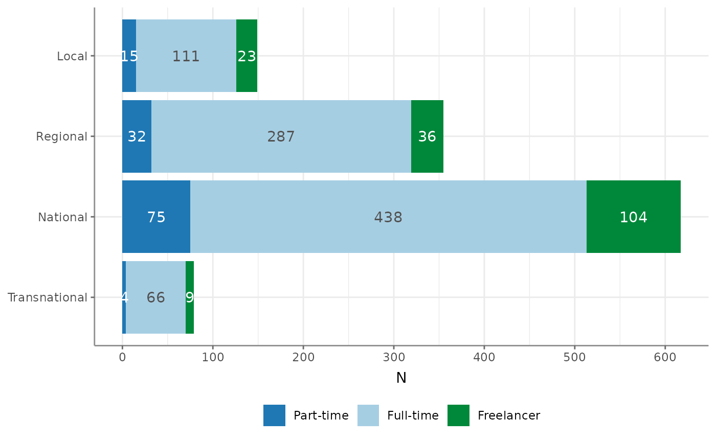
#> 15 Part-time  UK          0.00671  0.00563  0.00486        0.0506

You can also visualize the output from crosstab():

WoJ %>% 
  crosstab(reach, employment, percentages = TRUE) %>% 
  visualize()

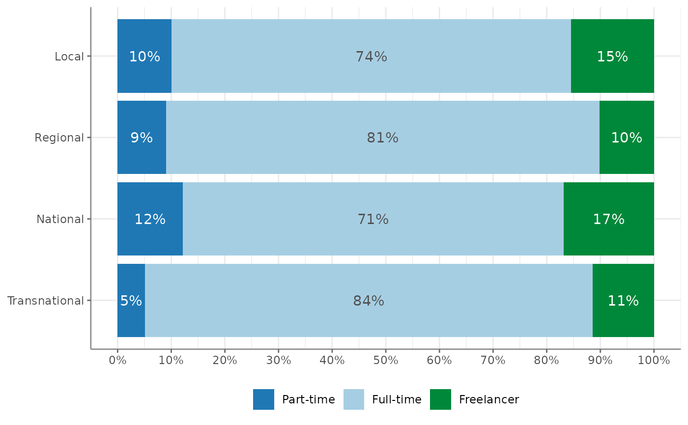
Note that the percentages = TRUE argument determines whether the bars add up to 100% and thus cover the whole width or whether they do not:

WoJ %>% 
  crosstab(reach, employment) %>% 
  visualize()

Compute t-Tests

Use t_test() to quickly compute t-Tests for a group variable and one or more test variables. Output includes test statistics, descriptive statistics and Cohen’s $d$ effect size estimates:

WoJ %>% 
  t_test(temp_contract, autonomy_selection, autonomy_emphasis)
#> # A tibble: 2 × 12
#>   Variable M_Permanent SD_Permanent M_Temporary SD_Temporary Delta_M     t    df
#> * <chr>      <num:.3!>    <num:.3!>   <num:.3!>    <num:.3!> <num:.> <num> <dbl>
#> 1 autonom…       3.910        0.755       3.698        0.932   0.212 1.627    56
#> 2 autonom…       4.124        0.768       3.887        0.870   0.237 2.171   995
#> # ℹ 4 more variables: p <num:.3!>, d <num:.3!>, Levene_p <dbl>, var_equal <chr>

Passing no test variables will compute t-Tests for all numerical variables in the data:

WoJ %>% 
  t_test(temp_contract)
#> # A tibble: 11 × 12
#>    Variable     M_Permanent SD_Permanent M_Temporary SD_Temporary Delta_M      t
#>  * <chr>          <num:.3!>    <num:.3!>   <num:.3!>    <num:.3!> <num:.> <num:>
#>  1 autonomy_se…       3.910        0.755       3.698        0.932   0.212  1.627
#>  2 autonomy_em…       4.124        0.768       3.887        0.870   0.237  2.171
#>  3 ethics_1           1.568        0.850       1.981        0.990  -0.414 -3.415
#>  4 ethics_2           3.241        1.263       3.509        1.234  -0.269 -1.510
#>  5 ethics_3           2.369        1.121       2.283        0.928   0.086  0.549
#>  6 ethics_4           2.534        1.239       2.566        1.217  -0.032 -0.185
#>  7 work_experi…      17.707       10.540      11.283       11.821   6.424  4.288
#>  8 trust_parli…       3.073        0.797       3.019        0.772   0.054  0.480
#>  9 trust_gover…       2.870        0.847       2.642        0.811   0.229  1.918
#> 10 trust_parti…       2.430        0.724       2.358        0.736   0.072  0.703
#> 11 trust_polit…       2.533        0.707       2.396        0.689   0.136  1.369
#> # ℹ 5 more variables: df <dbl>, p <num:.3!>, d <num:.3!>, Levene_p <dbl>,
#> #   var_equal <chr>

If passing a group variable with more than two unique levels, t_test() will produce a warning and default to the first two unique values. You can manually define the levels by setting the levels argument:

WoJ %>% 
  t_test(employment, autonomy_selection, autonomy_emphasis)
#> Warning: employment has more than 2 levels, defaulting to first two (Full-time
#> and Part-time). Consider filtering your data or setting levels with the levels
#> argument
#> # A tibble: 2 × 12
#>   Variable     `M_Full-time` `SD_Full-time` `M_Part-time` `SD_Part-time` Delta_M
#> * <chr>            <num:.3!>      <num:.3!>     <num:.3!>      <num:.3!> <num:.>
#> 1 autonomy_se…         3.903          0.782         3.825          0.633   0.078
#> 2 autonomy_em…         4.118          0.781         4.016          0.759   0.102
#> # ℹ 6 more variables: t <num:.3!>, df <dbl>, p <num:.3!>, d <num:.3!>,
#> #   Levene_p <dbl>, var_equal <chr>

WoJ %>% 
  t_test(employment, autonomy_selection, autonomy_emphasis, levels = c("Full-time", "Freelancer"))
#> # A tibble: 2 × 12
#>   Variable `M_Full-time` `SD_Full-time` M_Freelancer SD_Freelancer Delta_M     t
#> * <chr>        <num:.3!>      <num:.3!>    <num:.3!>     <num:.3!> <num:.> <num>
#> 1 autonom…         3.903          0.782        3.765         0.993   0.139 1.724
#> 2 autonom…         4.118          0.781        3.901         0.852   0.217 3.287
#> # ℹ 5 more variables: df <dbl>, p <num:.3!>, d <num:.3!>, Levene_p <dbl>,
#> #   var_equal <chr>

Additional options include:

pooled_sd: By default, the pooled variance will be used the compute Cohen’s $d$ effect size estimates ( $s = \sqrt\frac{(n_1 - 1)s^2_1 + (n_2 - 1)s^2_2}{n_1 + n_2 - 2}$ ). Set pooled_sd = FALSE to use the simple variance estimation instead ( $s = \sqrt\frac{(s^2_1 + s^2_2)}{2}$ ).
paired: Set paired = TRUE to compute a paired t-Test instead. It is advisable to specify the case-identifying variable with case_var when computing paired t-Tests, as this will make sure that data are properly sorted.

Previously, the (now deprecated) option of var.equal was also available. This has been overthrown, however, as t_test() now by default tests for equal variance (using a Levene test) to decide whether to use pooled variance or to use the Welch approximation to the degrees of freedom.

t_test() also provides a one-sample t-Test if you provide a mu argument:

WoJ %>% 
  t_test(autonomy_emphasis, mu = 3.9)
#> # A tibble: 1 × 9
#>   Variable              M    SD CI_95_LL CI_95_UL    Mu     t    df        p
#> * <chr>             <dbl> <dbl>    <dbl>    <dbl> <dbl> <dbl> <dbl>    <dbl>
#> 1 autonomy_emphasis  4.08 0.793     4.03     4.12   3.9  7.68  1194 3.23e-14

Of course, also the result from t-Tests can be visualized easily as such:

WoJ %>% 
  t_test(temp_contract, autonomy_selection, autonomy_emphasis) %>% 
  visualize()

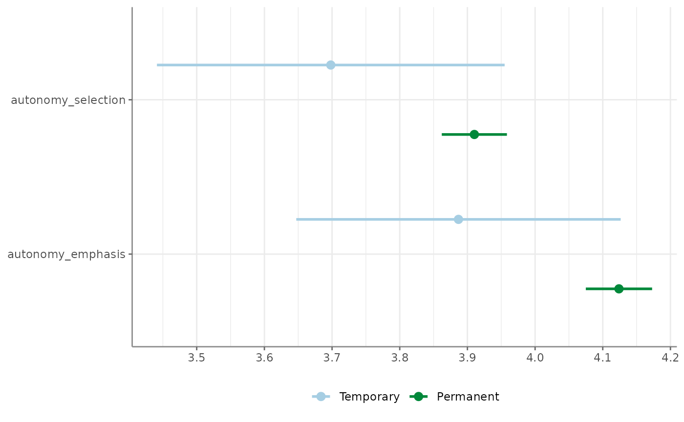
Compute one-way ANOVAs

unianova() will compute one-way ANOVAs for one group variable and one or more test variables. Output includes test statistics, $\eta^2$ effect size estimates, and $\omega^2$ , if Welch’s approximation is used to account for unequal variances.

WoJ %>% 
  unianova(employment, autonomy_selection, autonomy_emphasis)
#> # A tibble: 2 × 9
#>   Variable            F df_num df_denom     p omega_squared eta_squared Levene_p
#> * <chr>           <num>  <dbl>    <dbl> <num>     <num:.3!>   <num:.3!>    <dbl>
#> 1 autonomy_selec… 2.012      2      251 0.136         0.002      NA        0    
#> 2 autonomy_empha… 5.861      2     1192 0.003        NA           0.010    0.175
#> # ℹ 1 more variable: var_equal <chr>

Descriptives can be added by setting descriptives = TRUE. If no test variables are passed, all numerical variables in the data will be used:

WoJ %>% 
  unianova(employment, descriptives = TRUE)
#> # A tibble: 11 × 15
#>    Variable                  F df_num df_denom     p omega_squared `M_Full-time`
#>  * <chr>              <num:.3>  <dbl>    <dbl> <num>     <num:.3!>         <dbl>
#>  1 autonomy_selection    2.012      2      251 0.136         0.002          3.90
#>  2 autonomy_emphasis     5.861      2     1192 0.003        NA              4.12
#>  3 ethics_1              2.171      2     1197 0.115        NA              1.62
#>  4 ethics_2              2.204      2     1197 0.111        NA              3.24
#>  5 ethics_3              5.823      2      253 0.003         0.007          2.39
#>  6 ethics_4              3.453      2     1197 0.032        NA              2.58
#>  7 work_experience       3.739      2      240 0.025         0.006         17.5 
#>  8 trust_parliament      1.527      2     1197 0.218        NA              3.06
#>  9 trust_government     12.864      2     1197 0.000        NA              2.82
#> 10 trust_parties         0.842      2     1197 0.431        NA              2.42
#> 11 trust_politicians     0.328      2     1197 0.721        NA              2.52
#> # ℹ 8 more variables: `SD_Full-time` <dbl>, `M_Part-time` <dbl>,
#> #   `SD_Part-time` <dbl>, M_Freelancer <dbl>, SD_Freelancer <dbl>,
#> #   eta_squared <num:.3!>, Levene_p <dbl>, var_equal <chr>

You can also compute Tukey’s HSD post-hoc tests by setting post_hoc = TRUE. Results will be added as a tibble in a list column post_hoc.

WoJ %>% 
  unianova(employment, autonomy_selection, autonomy_emphasis, post_hoc = TRUE)
#> # A tibble: 2 × 10
#>   Variable            F df_num df_denom     p omega_squared post_hoc eta_squared
#> * <chr>           <num>  <dbl>    <dbl> <num>     <num:.3!> <list>     <num:.3!>
#> 1 autonomy_selec… 2.012      2      251 0.136         0.002 <df>          NA    
#> 2 autonomy_empha… 5.861      2     1192 0.003        NA     <df>           0.010
#> # ℹ 2 more variables: Levene_p <dbl>, var_equal <chr>

These can then be unnested with tidyr::unnest():

WoJ %>% 
  unianova(employment, autonomy_selection, autonomy_emphasis, post_hoc = TRUE) %>% 
  dplyr::select(Variable, post_hoc) %>% 
  tidyr::unnest(post_hoc)
#> # A tibble: 6 × 11
#>   Variable      Group_Var contrast Delta_M conf_lower conf_upper       p       d
#>   <chr>         <chr>     <chr>      <dbl>      <dbl>      <dbl>   <dbl>   <dbl>
#> 1 autonomy_sel… employme… Full-ti… -0.0780     -0.225     0.0688 0.422   -0.110 
#> 2 autonomy_sel… employme… Full-ti… -0.139      -0.329     0.0512 0.199   -0.155 
#> 3 autonomy_sel… employme… Part-ti… -0.0607     -0.284     0.163  0.798   -0.0729
#> 4 autonomy_emp… employme… Full-ti… -0.102      -0.278     0.0741 0.362   -0.133 
#> 5 autonomy_emp… employme… Full-ti… -0.217      -0.372    -0.0629 0.00284 -0.266 
#> 6 autonomy_emp… employme… Part-ti… -0.115      -0.333     0.102  0.428   -0.143 
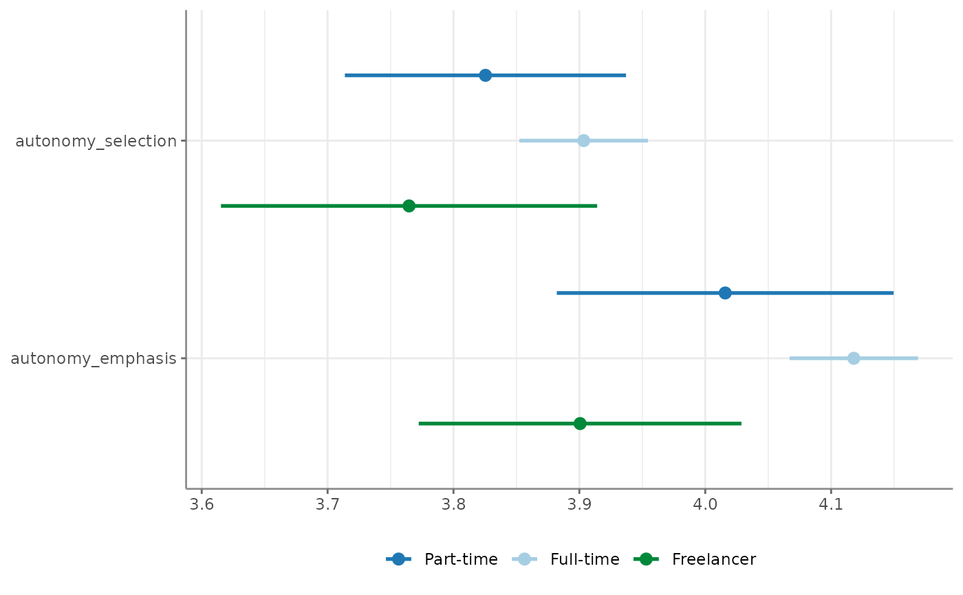
#> # ℹ 3 more variables: se <dbl>, t <dbl>, df <dbl>

Visualize one-way ANOVAs the way you visualize almost everything in tidycomm:

WoJ %>% 
  unianova(employment, autonomy_selection, autonomy_emphasis) %>% 
  visualize()

Compute correlation tables and matrices

correlate() will compute correlations for all combinations of the passed variables:

WoJ %>% 
  correlate(work_experience, autonomy_selection, autonomy_emphasis)
#> # A tibble: 3 × 6
#>   x                  y                      r    df         p     n
#> * <chr>              <chr>              <dbl> <int>     <dbl> <int>
#> 1 work_experience    autonomy_selection 0.161  1182 2.71e-  8  1184
#> 2 work_experience    autonomy_emphasis  0.155  1180 8.87e-  8  1182
#> 3 autonomy_selection autonomy_emphasis  0.644  1192 4.83e-141  1194

If no variables passed, correlations for all combinations of numerical variables will be computed:

WoJ %>% 
  correlate()
#> # A tibble: 55 × 6
#>    x                  y                        r    df         p     n
#>  * <chr>              <chr>                <dbl> <int>     <dbl> <int>
#>  1 autonomy_selection autonomy_emphasis  0.644    1192 4.83e-141  1194
#>  2 autonomy_selection ethics_1          -0.0766   1195 7.98e-  3  1197
#>  3 autonomy_selection ethics_2          -0.0274   1195 3.43e-  1  1197
#>  4 autonomy_selection ethics_3          -0.0257   1195 3.73e-  1  1197
#>  5 autonomy_selection ethics_4          -0.0781   1195 6.89e-  3  1197
#>  6 autonomy_selection work_experience    0.161    1182 2.71e-  8  1184
#>  7 autonomy_selection trust_parliament  -0.00840  1195 7.72e-  1  1197
#>  8 autonomy_selection trust_government   0.0414   1195 1.53e-  1  1197
#>  9 autonomy_selection trust_parties      0.0269   1195 3.52e-  1  1197
#> 10 autonomy_selection trust_politicians  0.0109   1195 7.07e-  1  1197
#> # ℹ 45 more rows

Specify a focus variable using the with parameter to correlate all other variables with this focus variable.

WoJ %>% 
  correlate(autonomy_selection, autonomy_emphasis, with = work_experience)
#> # A tibble: 2 × 6
#>   x               y                      r    df            p     n
#> * <chr>           <chr>              <dbl> <int>        <dbl> <int>
#> 1 work_experience autonomy_selection 0.161  1182 0.0000000271  1184
#> 2 work_experience autonomy_emphasis  0.155  1180 0.0000000887  1182

Run a partial correlation by designating three variables along with the partial parameter.

WoJ %>% 
  correlate(autonomy_selection, autonomy_emphasis, partial = work_experience)
#> # A tibble: 1 × 7
#>   x                  y                 z                 r    df         p     n
#> * <chr>              <chr>             <chr>         <dbl> <dbl>     <dbl> <int>
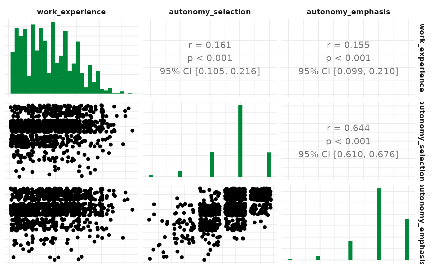
#> 1 autonomy_selection autonomy_emphasis work_experie… 0.637  1178 3.07e-135  1181

Visualize correlations by passing the results on to the visualize() function:

WoJ %>% 
  correlate(work_experience, autonomy_selection) %>% 
  visualize()

If you provide more than two variables, you automatically get a correlogram (the same you would get if you convert correlations to a correlation matrix):

WoJ %>% 
  correlate(work_experience, autonomy_selection, autonomy_emphasis) %>% 
  visualize()

By default, Pearson’s product-moment correlations coefficients ( $r$ ) will be computed. Set method to "kendall" to obtain Kendall’s $\tau$ or to "spearman" to obtain Spearman’s $\rho$ instead.

To obtain a correlation matrix, pass the output of correlate() to to_correlation_matrix():

WoJ %>% 
  correlate(work_experience, autonomy_selection, autonomy_emphasis) %>% 
  to_correlation_matrix()
#> # A tibble: 3 × 4
#>   r                  work_experience autonomy_selection autonomy_emphasis
#> * <chr>                        <dbl>              <dbl>             <dbl>
#> 1 work_experience              1                  0.161             0.155
#> 2 autonomy_selection           0.161              1                 0.644
#> 3 autonomy_emphasis            0.155              0.644             1

Compute linear regressions

regress() will create a linear regression on one dependent variable with a flexible number of independent variables. Independent variables can thereby be continuous, dichotomous, and factorial (in which case each factor level will be translated into a dichotomous dummy variable version):

WoJ %>% 
  regress(autonomy_selection, work_experience, trust_government)
#> # A tibble: 3 × 6
#>   Variable              B  StdErr    beta     t         p
#> * <chr>             <dbl>   <dbl>   <dbl> <dbl>     <dbl>
#> 1 (Intercept)      3.52   0.0906  NA      38.8  3.02e-213
#> 2 work_experience  0.0121 0.00211  0.164   5.72 1.35e-  8
#> 3 trust_government 0.0501 0.0271   0.0531  1.85 6.49e-  2
#> # F(2, 1181) = 17.400584, p = 0.000000, R-square = 0.028624

The function automatically adds standardized beta values to the expected linear-regression output. You can also opt in to calculate up to three precondition checks:

WoJ %>% 
  regress(autonomy_selection, work_experience, trust_government,
          check_independenterrors = TRUE,
          check_multicollinearity = TRUE,
          check_homoscedasticity = TRUE)
#> # A tibble: 3 × 8
#>   Variable              B  StdErr    beta     t         p   VIF tolerance
#> * <chr>             <dbl>   <dbl>   <dbl> <dbl>     <dbl> <dbl>     <dbl>
#> 1 (Intercept)      3.52   0.0906  NA      38.8  3.02e-213 NA       NA    
#> 2 work_experience  0.0121 0.00211  0.164   5.72 1.35e-  8  1.01     0.995
#> 3 trust_government 0.0501 0.0271   0.0531  1.85 6.49e-  2  1.01     0.995
#> # F(2, 1181) = 17.400584, p = 0.000000, R-square = 0.028624
#> - Check for independent errors: Durbin-Watson = 1.928431 (p = 0.244000)
#> - Check for homoscedasticity: Breusch-Pagan = 0.181605 (p = 0.669997)
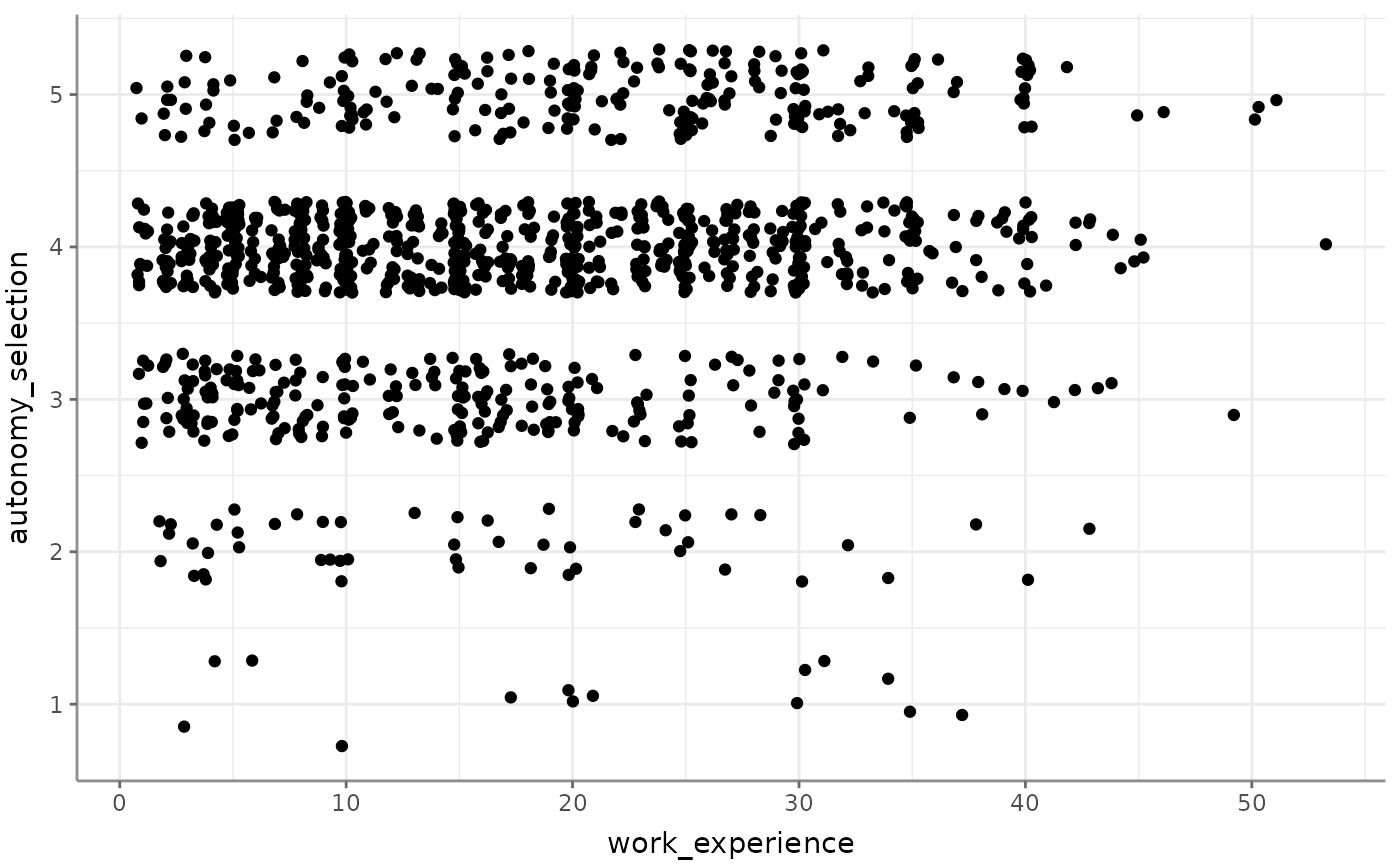
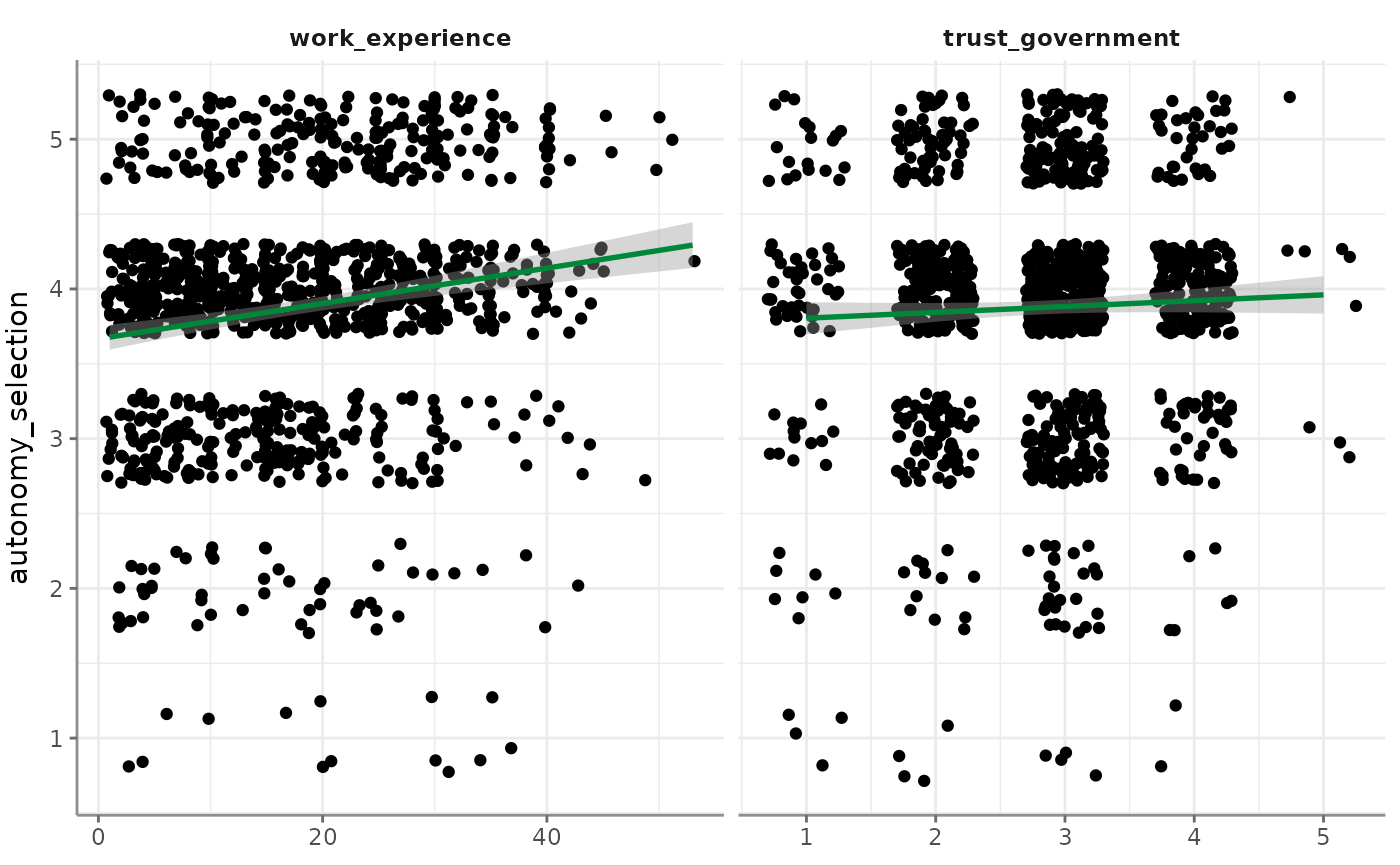
#> - Check for multicollinearity: VIF/tolerance added to output

For linear regressions, a number of visualizations are possible. The default one is the visualization of the result(s), is that the dependent variable is correlated with each of the independent variables separately and a linear model is presented in these:

WoJ %>% 
  regress(autonomy_selection, work_experience, trust_government) %>% 
  visualize()

Alternatively you can visualize precondition-check-assisting depictions. Correlograms among independent variables, for example:

WoJ %>% 
  regress(autonomy_selection, work_experience, trust_government) %>% 
  visualize(which = "correlogram")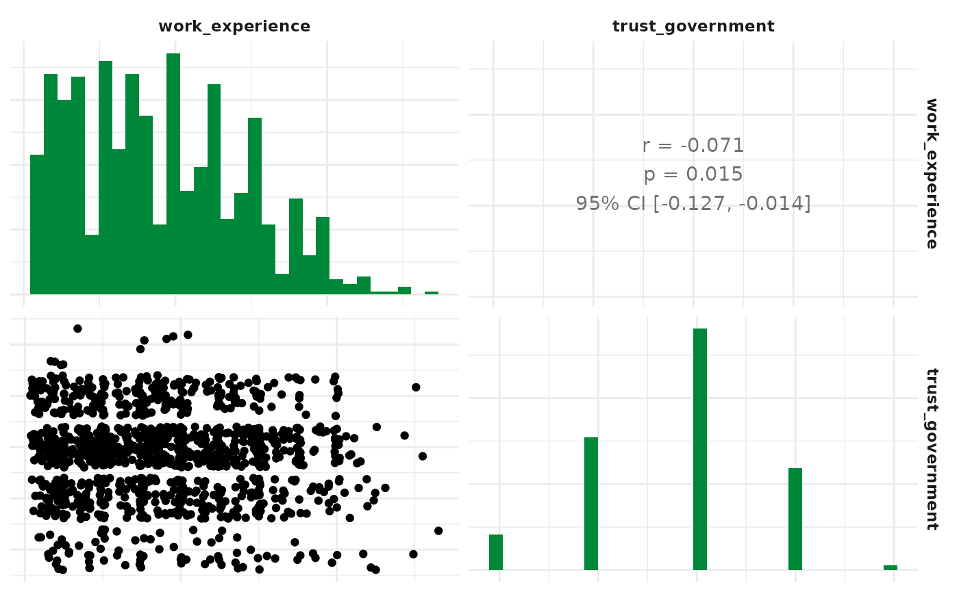

Next up, visualize a residuals-versus-fitted plot to determine distributions:

WoJ %>% 
  regress(autonomy_selection, work_experience, trust_government) %>% 
  visualize(which = "resfit")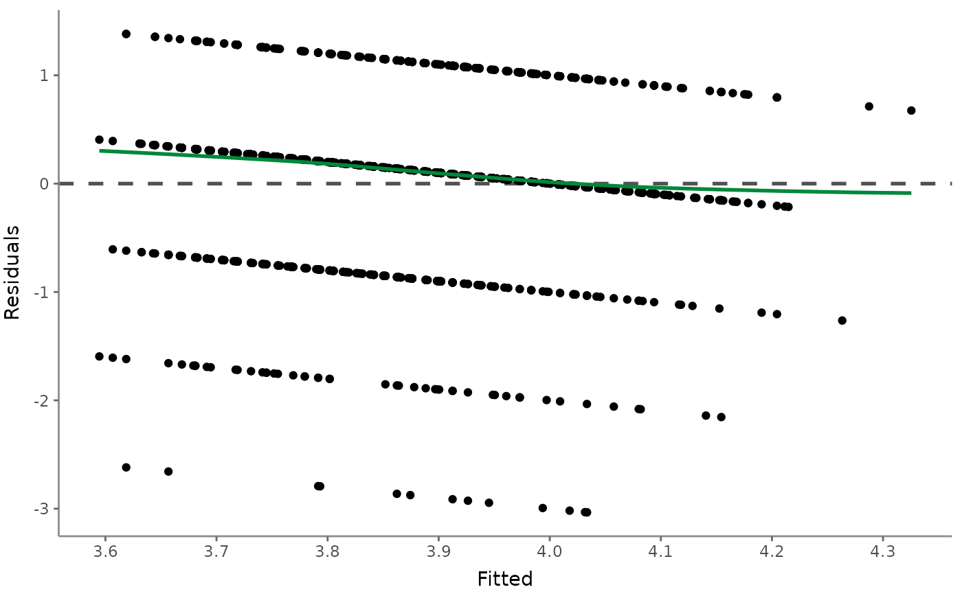

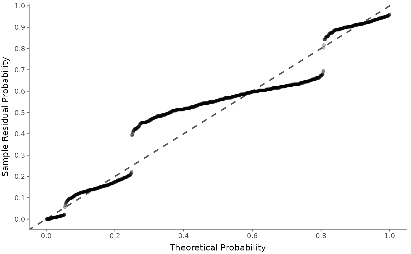
Or use a (normal) probability-probability plot to check for multicollinearity:

WoJ %>% 
  regress(autonomy_selection, work_experience, trust_government) %>% 
  visualize(which = "pp")

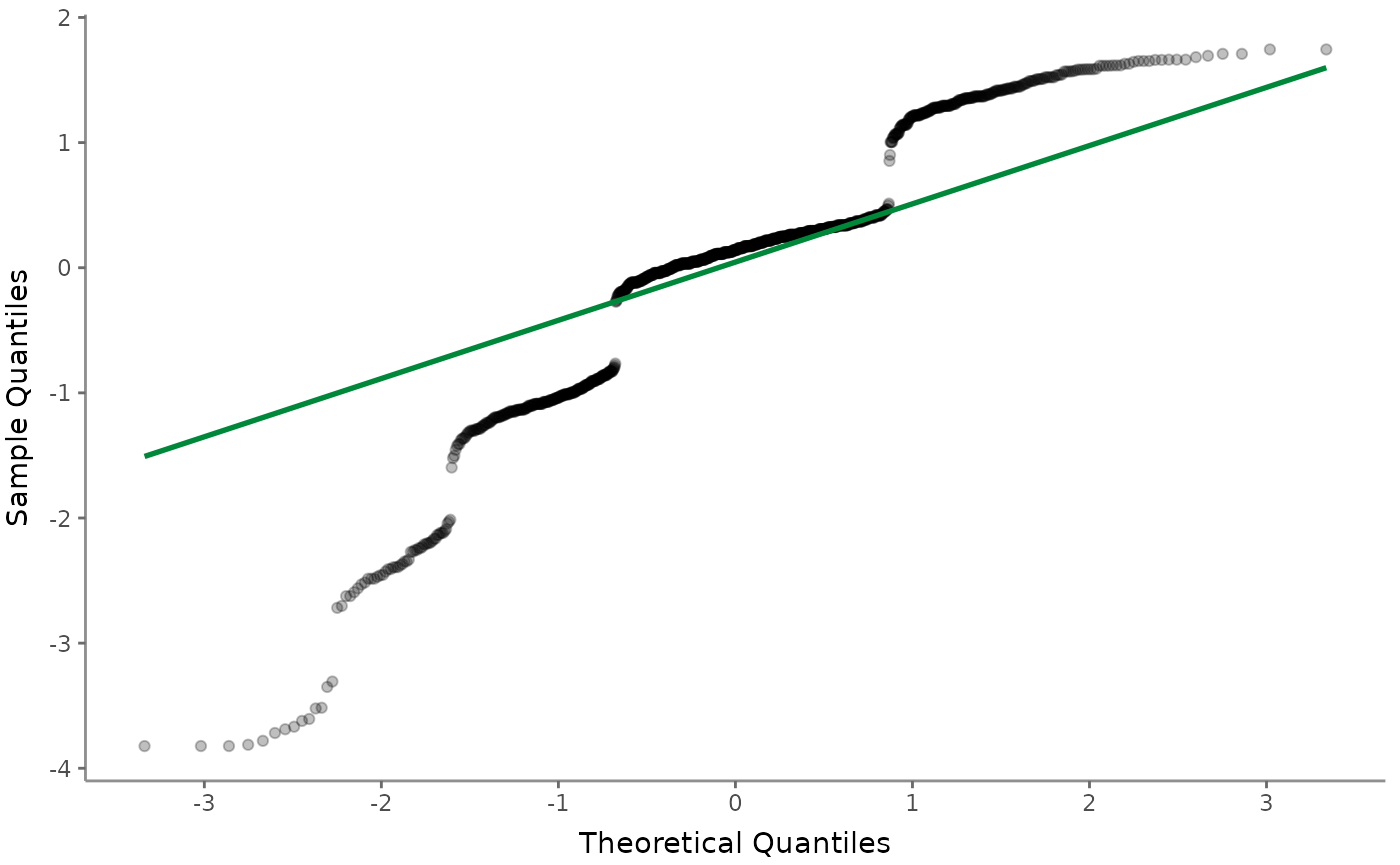
The (normal) quantile-quantile plot also helps checking for multicollinearity but focuses more on outliers:

WoJ %>% 
  regress(autonomy_selection, work_experience, trust_government) %>% 
  visualize(which = "qq")

Next up, the scale-location (sometimes also called spread-location) plot checks whether residuals are spread equally to help check for homoscedasticity:

WoJ %>% 
  regress(autonomy_selection, work_experience, trust_government) %>% 
  visualize(which = "scaloc")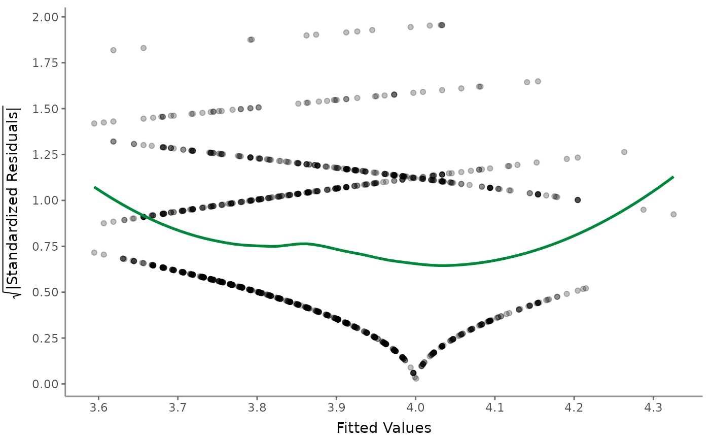

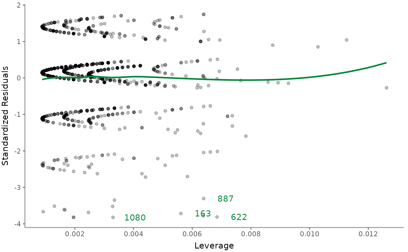
Finally, visualize the residuals-versus-leverage plot to check for influential outliers affecting the final model more than the rest of the data:

WoJ %>% 
  regress(autonomy_selection, work_experience, trust_government) %>% 
  visualize(which = "reslev")

2025-08-25

Compute contingency tables and Chi-square tests

Compute t-Tests

Compute one-way ANOVAs

Compute correlation tables and matrices

Compute linear regressions